Introduction: From Statics to Dynamics | Class 12 Physics Chapter 3 Current Electricity Notes

Welcome, students, to one of the most practical and essential chapters in Physics: Current Electricity. In our previous studies of Chapters 1 and 2, we focused entirely on Electrostatics. There, we treated electric charges as if they were frozen in time. We calculated the forces they exerted on each other and the potential energy they stored, but they never moved continuously.

Now, imagine releasing those charges. Just as water stored in a high tank flows down through a pipe when a tap is opened, electric charges will flow if given a path and a potential difference. This flow of charge is what we call Electric Current. In nature, we see this in dramatic, uncontrolled bursts like lightning, where charges jump from clouds to the earth through the atmosphere. However, for useful technology—like the device you are reading this on, or the lights in your room—we need the flow to be steady and controlled.

In this chapter, we will explore the laws governing these steady currents. We will understand why wires get hot, how batteries push electrons, and the complex rules that govern circuits. This is the foundation of modern electronics. Let’s begin!

1. Electric Current: The Fundamental Flow

1.1 Defining Electric Current

At its core, electric current is simply the rate at which electric charge flows through a specific area. Imagine a cross-section of a wire. If charges are moving through this wire, we count how much charge passes this cross-section in a specific time interval.

Mathematical Definition:
Let’s say a net charge $\Delta Q$ flows across a cross-section of a conductor during a time interval $\Delta t$. The average current $I_{avg}$ is defined as:
$$I_{avg} = \frac{\Delta Q}{\Delta t}$$
However, currents vary with time. To be precise, we define instantaneous current $I(t)$ as the limit of this ratio as time approaches zero:
$$I = \lim_{\Delta t \to 0} \frac{\Delta Q}{\Delta t} = \frac{dQ}{dt}$$

Units and Scales:
The SI unit of current is the Ampere (A). One Ampere is defined as one Coulomb of charge passing per second ($1 A = 1 C/s$).
To give you a sense of scale:

• Domestic Appliances: Your fridge or TV might draw a current of a few amperes (e.g., 1-5 A).
• Lightning: A lightning strike is massive, carrying tens of thousands of amperes.
• Human Body: Our nerves operate on tiny currents, in the range of microamperes ($\mu A$).

1.2 Direction of Current: A Historical Convention

This is a point of confusion for many students. By convention, the direction of electric current is taken as the direction of the flow of positive charges.

However, in metallic conductors (like copper wires), the positive ions are fixed in place. The only things moving are the negatively charged electrons. Therefore, the actual flow of charge carriers (electrons) is opposite to the conventional direction of current.

Teacher’s Tip: Always draw current arrows from Positive (+) to Negative (-) in a circuit, even though you know electrons are running the other way!.

1.3 Current Density (j)

Current ($I$) is a macroscopic quantity—it tells us the total flow. But sometimes, we want to know how crowded the flow is at a specific microscopic point. For this, we use a vector quantity called Current Density ($j$).

Current Density is defined as the current per unit area (taken normal to the current).
$$j = \frac{I}{A}$$
Since current flows in a specific direction driven by the electric field ($E$), current density is a vector directed along $E$. The relationship is:
$$j = \sigma E$$
where $\sigma$ is the conductivity of the material.

2. Mechanism of Conduction: The Drift of Electrons

To truly understand electricity, we must zoom in to the atomic level. What is happening inside a copper wire?

2.1 Case 1: No Electric Field (The Chaos)

Inside a metal, electrons are free to move. However, they are not sitting still. They are moving randomly at incredibly high speeds (thermal velocities) due to the temperature of the room. They constantly collide with the heavy, fixed positive ions of the metal lattice.

After each collision, an electron bounces off in a random direction. Because this motion is completely random, the average velocity of all electrons is zero. There is no net flow in any direction, and thus, no current.
$$\frac{1}{N} \sum_{i=1}^{N} v_i = 0$$

2.2 Case 2: With Electric Field (The Drift)

Now, imagine we connect a battery. This creates an Electric Field ($E$) inside the wire. This field exerts a force $F = -eE$ on every electron.

This force causes the electrons to accelerate.
$$a = \frac{F}{m} = -\frac{eE}{m}$$
However, they don’t just keep accelerating indefinitely like a rocket. They still collide with the fixed ions. The electric field gently pushes them towards the positive end, while the collisions scatter them.

The result is that, on top of their random chaotic motion, the electrons acquire a very small average velocity in the direction opposite to the field. This small, steady speed is called Drift Velocity ($v_d$).

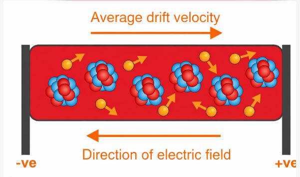
Figure-1: The solid line represents the random path of an electron. The dashed line shows how the path shifts (drifts) when an electric field is applied.

2.3 Derivation of Drift Velocity

Consider an electron. Let $\tau$ (tau) be the Relaxation Time—the average time between two successive collisions.
The velocity gained by an electron due to acceleration $a$ in time $\tau$ is:
$$v_d = a \tau$$
Substituting the value of acceleration $a = -eE/m$:
$$v_d = -\frac{eE}{m}\tau$$
(The negative sign indicates drift is opposite to the field).

2.4 Relation Between Current and Drift Velocity

This is one of the most important derivations for your board exams.

Consider a wire of cross-section $A$ and length $L$.
Let $n$ be the number density of free electrons (electrons per unit volume).

Total volume of the wire section = $A \times (v_d \Delta t)$ (distance covered in time $\Delta t$).
Total number of electrons = $n \times Volume = n A v_d \Delta t$.
Total Charge $\Delta Q = (n A v_d \Delta t) \times e$.

Current $I = \frac{\Delta Q}{\Delta t}$.
$$I = n A e v_d$$
This equation links the macroscopic current ($I$) to the microscopic drift velocity ($v_d$).

3. Ohm’s Law: The Rule of Resistance

In 1828, Georg Simon Ohm discovered a fundamental relationship. He found that for most conductors (like metals), the current ($I$) flowing through them is directly proportional to the potential difference ($V$) applied across them, provided the temperature remains constant.

$$V \propto I$$
$$V = R I$$
Here, the constant of proportionality $R$ is called Resistance. The SI unit is the Ohm ($\Omega$).

3.1 Factors Affecting Resistance

Resistance is essentially the opposition to current flow caused by collisions. It depends on the dimensions of the conductor:

• Length ($l$): A longer wire offers more collisions, so $R \propto l$.
• Area ($A$): A wider wire allows more electrons to pass simultaneously, so $R \propto 1/A$.

Combining these:
$$R = \rho \frac{l}{A}$$
Here, $\rho$ (rho) is the Resistivity. Resistivity is a property of the material itself (e.g., Copper, Iron, Rubber) and does not depend on the shape or size of the wire.

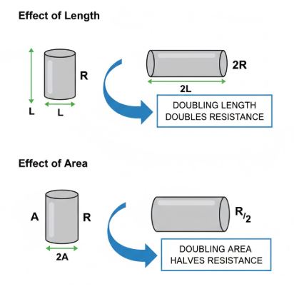
Figure-2: Visualizing Resistance: (a) Doubling length doubles resistance. (b) Doubling area halves resistance.

3.2 Vector Form of Ohm’s Law

We can express Ohm’s law at a microscopic level.
From $V = IR$, substituting $V=El$, $I=jA$, and $R = \rho l/A$:
$$El = (jA) (\rho \frac{l}{A})$$
$$E = j \rho$$
or
$$j = \sigma E$$
where $\sigma = 1/\rho$ is the Conductivity. This vector form tells us that current density is driven by and parallel to the electric field at every point.

3.3 Limitations of Ohm’s Law

Is Ohm’s law universal? No. It is not a fundamental law of nature like Newton’s laws. It is an empirical rule that works for many materials (Ohmic conductors) but fails for others (Non-Ohmic conductors).

Deviations include:

• Non-Linearity: In devices like diodes, the graph of $V$ vs $I$ is not a straight line.
• Direction Dependence: In a diode, current flows easily in one direction but not the other, meaning reversing $V$ does not just reverse $I$.
• Multiple Values: In materials like Gallium Arsenide (GaAs), there can be more than one value of $V$ for the same current $I$.

4. Resistivity and Temperature

Resistivity is not constant; it changes with temperature. The behavior is different for different classes of materials.

4.1 Metals (Conductors)

In metals, the number density of free electrons ($n$) is huge and doesn’t change much with temperature. However, as temperature rises, the ions in the lattice vibrate more vigorously.

Result: Electrons collide more frequently. The relaxation time ($\tau$) decreases. Since resistivity $\rho \propto 1/\tau$, the resistivity increases with temperature.

Formula:
$$\rho_T = \rho_0 [1 + \alpha(T – T_0)]$$
where $\alpha$ is the temperature coefficient of resistivity. For metals, $\alpha$ is positive.

4.2 Semiconductors (Si, Ge)

In semiconductors, the situation is different. At higher temperatures, thermal energy breaks covalent bonds, freeing up more electrons. The number density ($n$) increases drastically.

Result: This increase in charge carriers dominates the collision effect. Therefore, resistivity decreases as temperature increases. For semiconductors, $\alpha$ is negative.

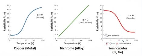
Figure-3: (Left) Resistivity of Copper increases non-linearly at low temps. (Center) Nichrome increases linearly. (Right) Semiconductor resistivity drops with temperature.

4.3 Alloys (Nichrome, Manganin)

Alloys like Manganin and Constantan are special. Their resistance changes very little with temperature. This property makes them ideal for making “Standard Resistors” for laboratory experiments, as their value won’t drift as the room warms up.

5. Electrical Energy and Power

Why do we pay electricity bills? We pay for energy. When current flows through a resistor, the charges lose potential energy. Where does this energy go? It is dissipated as heat (thermal energy).

Consider a current $I$ flowing across a potential difference $V$ for time $\Delta t$.
The charge transported is $\Delta Q = I \Delta t$.
The work done (potential energy lost) is:
$$Work = V \times \Delta Q = V I \Delta t$$
This energy is converted into heat.

Electric Power:
Power is the rate of energy consumption ($P = W/t$).
$$P = V I$$
Using Ohm’s law ($V=IR$), we can write:
$$P = I^2 R = \frac{V^2}{R}$$

Real-Life Application: High Voltage Transmission
You might have seen “High Voltage” signs on power pylons. Why do we transmit power at such dangerous voltages?

Power loss in wires is given by $I^2 R_c$ (where $R_c$ is cable resistance). To minimize loss, we need to minimize Current ($I$). Since Power delivered $P = VI$, to keep $P$ constant while reducing $I$, we must increase Voltage ($V$) enormously. This is why grid power is transmitted at thousands of volts before being stepped down by transformers for your home.

6. Cells, EMF, and Internal Resistance

A wire creates resistance, but what pushes the current? A “Cell” or “Battery”.
Imagine a cell as a pump that lifts charges from low potential to high potential, using chemical energy.

6.1 Electromotive Force (EMF)

The term Electromotive Force ($\varepsilon$) is a historical misnomer. It is NOT a force.

Definition: EMF is the potential difference between the two terminals of a cell when the circuit is open (i.e., no current is flowing). It represents the maximum voltage the cell can deliver.

6.2 Internal Resistance (r)

Inside a cell, ions move through an electrolyte. The electrolyte offers some resistance to this motion. This is called the Internal Resistance ($r$) of the cell. Ideally, $r$ should be zero, but real cells always have finite internal resistance.

6.3 Terminal Voltage (V)

When you connect the cell to a circuit and draw current $I$, the potential difference across the terminals drops. Why? Because some voltage is “lost” in overcoming the internal resistance ($Ir$).

The relationship is:
$$V = \varepsilon – I r$$
Or, $I = \frac{\varepsilon}{R + r}$ (where $R$ is external resistance).

7. Grouping of Cells

Just like resistors, we can connect multiple cells to get more voltage or more current.

7.1 Cells in Series

When negative terminal of one cell is connected to the positive of the next:

• Equivalent EMF: $\varepsilon_{eq} = \varepsilon_1 + \varepsilon_2 + \dots$ (Voltages add up).
• Equivalent Internal Resistance: $r_{eq} = r_1 + r_2 + \dots$ (Resistances add up).

Note: If a cell is connected with wrong polarity (positive to positive), its EMF is subtracted ($\varepsilon_1 – \varepsilon_2$).

7.2 Cells in Parallel

When all positive terminals are connected to one point and all negatives to another:

• Equivalent EMF: $\frac{\varepsilon_{eq}}{r_{eq}} = \frac{\varepsilon_1}{r_1} + \frac{\varepsilon_2}{r_2} + \dots$.
• Equivalent Internal Resistance: $\frac{1}{r_{eq}} = \frac{1}{r_1} + \frac{1}{r_2} + \dots$.

For two cells, this simplifies to: $\varepsilon_{eq} = \frac{\varepsilon_1 r_2 + \varepsilon_2 r_1}{r_1 + r_2}$.

8. Kirchhoff’s Rules: Solving Complex Circuits

Ohm’s law is great for simple loops. But what if you have a complex mesh of wires like a spider web? Gustav Kirchhoff gave us two powerful rules to solve any electrical network.

Rule 1: The Junction Rule (Current Law)

Statement: At any junction (node), the sum of currents entering equals the sum of currents leaving.
$$\sum I_{in} = \sum I_{out}$$
Physics Principle: Conservation of Charge. Charges cannot pile up at a point, nor can they be created out of thin air. Whatever flows in must flow out.

Rule 2: The Loop Rule (Voltage Law)

Statement: The algebraic sum of changes in potential around any closed loop involving resistors and cells is zero.
$$\sum \Delta V = 0$$
Physics Principle: Conservation of Energy. Electric potential is related to energy. If you start at a point in a circuit (say, potential 5V) and go around a loop back to the same point, the potential must be 5V again. The net change must be zero.

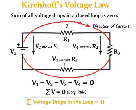
Figure-4: (a) Currents at a junction. (b) Traversing a closed loop to sum voltages.

Sign Convention (Crucial for Numericals):

• Traversing resistor in direction of current: Potential Drops ($-IR$).
• Traversing resistor opposite to current: Potential Rises ($+IR$).
• Traversing cell from Negative to Positive: Potential Rises ($+\varepsilon$).
• Traversing cell from Positive to Negative: Potential Drops ($-\varepsilon$).

9. The Wheatstone Bridge

This is a very clever application of Kirchhoff’s laws used to measure an unknown resistance very precisely. It consists of 4 resistors arranged in a quadrilateral, with a battery across one diagonal and a galvanometer (current detector) across the other.

9.1 The Balanced Condition

We adjust the values of the resistors until the Galvanometer shows Zero Deflection ($I_g = 0$). This is called the “Null Point”.

When the bridge is balanced, no current flows between points B and D. This implies:

1. Potential at B = Potential at D.
2. Current divides such that the ratio of arms is equal.

Derivation:
Using Kirchhoff’s loop rule on the two loops when $I_g = 0$:
Loop 1: $-I_1 R_1 + I_2 R_2 = 0 \implies I_1 R_1 = I_2 R_2$
Loop 2: $I_2 R_4 – I_1 R_3 = 0 \implies I_1 R_3 = I_2 R_4$
Dividing the two equations:
$$\frac{R_2}{R_1} = \frac{R_4}{R_3}$$
This is the condition for a balanced Wheatstone bridge.

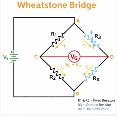
Figure-5: Wheatstone Bridge. When balanced, the galvanometer G reads zero current.

Practical Uses:
The Meter Bridge is a practical laboratory device based on this principle used to find the resistance of a given wire.

Comprehensive Solved Numericals

Numerical 1: Drift Velocity Calculation

Q: A copper wire of cross-sectional area $1.0 \times 10^{-7} m^2$ carries a current of 1.5 A. Calculate the drift velocity. (Density of free electrons $n = 8.5 \times 10^{28} m^{-3}$).

Solution:
We use the formula: $I = n A e v_d$.
Rearranging for drift velocity: $v_d = \frac{I}{nAe}$.
Given:
$I = 1.5 \, A$
$n = 8.5 \times 10^{28} \, m^{-3}$
$A = 1.0 \times 10^{-7} \, m^2$
$e = 1.6 \times 10^{-19} \, C$
Substitute values:
$v_d = \frac{1.5}{(8.5 \times 10^{28}) (1.0 \times 10^{-7}) (1.6 \times 10^{-19})}$
$v_d = \frac{1.5}{13.6 \times 10^2} = 1.1 \times 10^{-3} \, m/s = 1.1 \, mm/s$.
Interpretation: Electrons drift incredibly slowly—about 1 mm per second!

Numerical 2: Temperature Effect

Q: A heating element has a resistance of $75.3 \Omega$ at $27^\circ C$. When connected to 230V, the current settles at 2.68 A. If $\alpha = 1.70 \times 10^{-4} C^{-1}$, find the steady temperature.

Solution:
Step 1: Find resistance at steady temp ($R_2$).
$R_2 = V/I = 230 / 2.68 = 85.8 \Omega$.
Step 2: Use temperature formula.
$R_2 = R_1 [1 + \alpha (T_2 – T_1)]$.
$85.8 = 75.3 [1 + 1.7 \times 10^{-4} (T_2 – 27)]$.
$\frac{85.8}{75.3} – 1 = 1.7 \times 10^{-4} (T_2 – 27)$.
$0.139 = 1.7 \times 10^{-4} (T_2 – 27)$.
$T_2 – 27 = \frac{0.139}{0.00017} \approx 820$.
$T_2 = 847^\circ C$.

Numerical 3: Internal Resistance

Q: A battery of EMF 10 V and internal resistance $3 \Omega$ is connected to a resistor. If the current is 0.5 A, calculate the resistance of the resistor and the terminal voltage.

Solution:
Formula: $I = \frac{\varepsilon}{R+r}$.
$0.5 = \frac{10}{R+3}$.
$0.5(R+3) = 10 \Rightarrow R+3 = 20 \Rightarrow R = 17 \Omega$.
Terminal Voltage $V = I R = 0.5 \times 17 = 8.5 V$.
(Alternatively, $V = \varepsilon – Ir = 10 – (0.5 \times 3) = 10 – 1.5 = 8.5 V$).

CBSE Board Extensive Practice Set

Very Short Answer (1 Mark)

Q1. Define Mobility of a charge carrier. What is its SI unit?
Ans: Mobility ($\mu$) is defined as the magnitude of drift velocity per unit electric field: $\mu = |v_d|/E$. Its SI unit is $m^2 V^{-1} s^{-1}$.

Q2. Two wires of equal length and diameter are made of Copper and Nichrome. Which one has higher resistance?
Ans: Nichrome. It is an alloy with much higher resistivity than pure copper.

Q3. Why are connecting wires in a circuit made of thick copper?
Ans: To minimize resistance. $R \propto 1/A$, so thick wires have lower resistance, reducing voltage drop and power loss in the wires.

Short Answer (2-3 Marks)

Q4. Explain the concept of “Relaxation Time” and how it relates to drift velocity.
Ans: Relaxation time ($\tau$) is the average time interval between two successive collisions of an electron with the positive ions in the conductor. Drift velocity is directly proportional to relaxation time ($v_d = \frac{eE}{m}\tau$). If $\tau$ decreases (e.g., due to heating), drift velocity decreases.

Q5. State Kirchhoff’s Junction Rule. Show that it is based on the law of conservation of charge.
Ans: The rule states that the algebraic sum of currents meeting at a junction is zero ($\sum I = 0$). This means total current entering equals total current leaving. Since current is the flow of charge per unit time, this implies that charge is not accumulating or disappearing at the junction, which is the conservation of charge.

Long Answer (5 Marks)

Q6. (a) Define Drift Velocity. Derive the expression $I = n A e v_d$.
(b) A potential difference $V$ is applied to a conductor of length $L$. How is drift velocity affected if $V$ is doubled and $L$ is halved?
Ans: (a) Drift velocity is the average velocity acquired by electrons in the presence of an external electric field. (See derivation in Section 2.4).
(b) We know $v_d = \frac{eE}{m}\tau$. Also, Electric field $E = V/L$.
So, $v_d = \frac{e V \tau}{m L}$.
If $V$ becomes $2V$ and $L$ becomes $L/2$:
New $v_d’ = \frac{e (2V) \tau}{m (L/2)} = 4 \left(\frac{e V \tau}{m L}\right) = 4 v_d$.
Thus, the drift velocity becomes 4 times the original value.

Case-Based Question (4 Marks)

Q7. The Car Battery
A student notices that when he tries to start his car, the headlights dim significantly for a moment. He knows the car battery has an EMF of 12V. He measures the internal resistance to be $0.05 \Omega$. The starter motor draws a massive current of 80A.
(i) What is the terminal voltage of the battery when the starter is running?
(ii) Why do the lights dim?
(iii) What is the maximum current this battery can theoretically provide?
Ans:
(i) Terminal Voltage $V = \varepsilon – I r = 12 – (80 \times 0.05) = 12 – 4 = 8 V$.
(ii) The lights dim because the voltage across them drops from 12V to 8V due to the heavy internal voltage drop ($Ir$) inside the battery.
(iii) Max current is when external resistance is zero (short circuit). $I_{max} = \varepsilon / r = 12 / 0.05 = 240 A$.